gCOSY

The Gradient-Selected COSY (gCOSY) Experiment

This Handout covers VnmrJ3.2A.

COrrelation SpectroscopY (COSY) is a 2D NMR technique that gives correlations between J-coupled signals by incrementing the delay between two 90º-proton pulses (see pulse sequence below). The resulting 2D spectrum is generally displayed as a contour plot, which is similar to a topographical map. When looking at a contour map, you are actually looking down at a cross-section (slice) of a 3D-image (two frequency and one intensity domain) of an NMR spectrum. The usual 1D spectrum is traced on the diagonal of the plot and any peaks that are not on the diagonal represent cross-peaks or correlation peaks that are a result of J-coupling. Thus, by simply tracing a rectangle using the diagonal and cross-peaks as vertices you will know which protons are coupled to each other. Standard COSY experiments require phase cycling to remove unwanted signals and thus can be quite time consuming. This can be largely circumvented using gradient-selected COSY (gCOSY), which utilizes pulsed field gradients to destroy unwanted magnetization and hence their associated signals (axial peaks). Quality gCOSY spectra can be acquired in as little as 5 minutes!

 

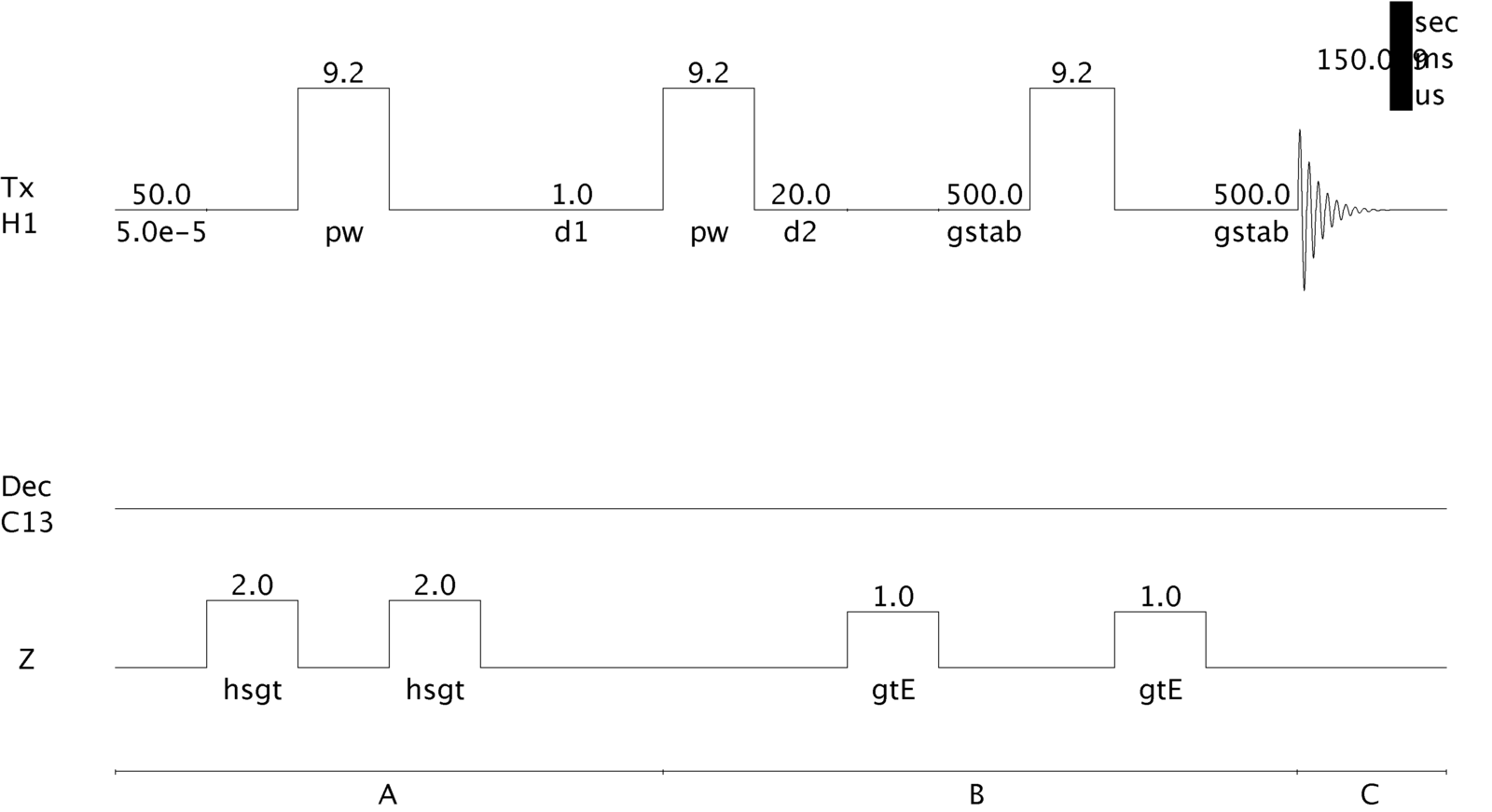
gCOSY Pulse Sequence as Implemented on a Varian Inova 500 MHz Spectrometer.

Please follow a few simple house rules:

1. Observe all operational procedures carefully.
2. If there is something that you don't know or are not sure about, please ask.
3. Use common sense and don't rush -- this will go a long way in avoiding costly mistakes.
4. Report any problem to Lab Staff.

Explanation of Types of Commands Found in this Handout:

1. The VNMR software and the UNIX operating system are both case sensitive. This means that the computer distinguishes whether the letters are entered in upper case (i.e. CAPITALS) or lower case. The user must be careful to type the correct case for each letter in a command.

   Example: jexp1 is not the same as JEXP1

2. Some commands are line commands and are typed in by the user followed by a return (a Return is assumed for typed bold text commands).

   Example: su

3. Parameters are entered by typing the parameter name followed by a equal sign, the value, and a return.

   Example: nt=16

If you have any problems or if you find any errors as you go through this handout, please let me know.

Daniel Holmes
Max T. Rogers NMR Facility

Running a gCOSY Experiment

To simplify use, please make sure that you have only 1 viewport enabled. Click Edit, Viewports… Select 1 for the Number of Viewports. Click Close.

Acquire a Standard ¹H Spectrum

Instructions	Explanation
type jexp1	join experiment 1
Insert your sample, lock, shim well, acquire, and process a standard 1D Proton spectrum. Note the left-most and right-most peaks from your spectrum (for example, 8 and 2 ppm) and decrease the Spectral Width to 1 ppm larger on either side (e.g. 9 and 1 ppm). This is gone in Default H1 of the Acquire tab of the Parameter panel. Rerun the Proton experiment with the new Spectral width.
type svf('filename')	save the FID

Setup the gCOSY Experiment

Instructions	Explanation
type jexp2	This joins experiment 2. If you get an error message, click File => New Workspace
type mf(1,2)	This moves the FID from exp1 to exp2
Turn off the spin and adjust the lock level to 80% or higher using lockgain and lockpower. Be sure not to saturate your lock signal with too high lock power. The lock power is too high if the lock level has large fluctuations or begins to decrease with increased lock power. NOTE: Turning off spinning is very important. You will not get good spectra if the sample is spinning because the gradients rely on the spatial stability of the nuclear spins! Click Experiments, Homonuclear Correlations, Gradient COSY. In the Defaults panel of the Acquire tab, select the number of Scans per t1 Increment (minimum of 4 is recommended) and number of t1 Increments (minimum of 128 is recommended). In general, increase Scans per t1 Increment for dilute samples or compounds with small 1H-1H coupling constants. Increase t1 Increments for crowded spectra.

Acquire a gCOSY spectrum

Instructions	Explanation
typego (do not type ga)	acquires 2D spectrum
Data Manipulation
type svf(‘filename’)	save 2D dataset.
type setLP1	sets linear predication in the indirectly detected dimension
NOTE: This will predict data to 3 times the length of your acquired data and gives apparent ‘better resolution’. If, after transforming your 2-D dataset, you suspect that this has created artifacts that clutter your spectrum, you can turn it off by typing proc1=’ft’. You will need to reprocess your data using wft2d.
type sinebell wft2d	This performs a sine bell apodization and a 2-dimensional Fourier transform and the color map will be displayed. The color map is your 2-D spectrum with the levels displayed using different colors. Use the following table as a guide to color map navigation.
Optional (type foldt)	This performs a symmetrization about the diagonal. It can make data look cleaner and easier to interpret. Be careful, however, as it can remove peaks that do not have a partner on the opposite side of the diagonal and can make noise appear to be a cross-peak.

Printing your Spectra

Printing your gCOSY with 1-D Spectrum as Projections (preferred method)

Instructions	Explanation
Click View, Parameter Panel	opens Parameter Panel
Click the Process Tab	opens Process Pane
Click Display	opens Display options
Under Screen Position, click Center
type jexp1	join another experiment
Load the 1-D spectrum (if necessary); Fourier transform (wft), and phase (aph).
type jexp2	join the experiment with your COSY
VnmrJ: Click in the top right	Displays contour map. By default, the number of levels is 4. To increase, please refer to the table on the following page for VnmrJ
Expand, scale, etc. the region of interest (refer to table for interacting with the color or contour map).

Interacting with the 2-D Color Map/Contour Map for VnmrJ

To do the following...	You should...
Increase/Decrease the scale	Scroll the mouse wheel to change height. Alternatively, click on either to increase or to decrease scale.
To expand on a region	Click on . Click on where you want to start to expand and drag to cover the desired expansion area.
To Pan & Stretch	Click . Click on the spectrum and drag to move to new area. Clicking and holding the right mouse button will allow you to expand or contract the spectrum.
To display full 2D spectrum	Click.
To expand an exact region	Type sp=#p wp=#p (for the F2 dimension, usually vertical) and sp1=#p wp1=#p (for the F1 dimension, usually horizontal), where # are the numbers in ppm for the region of interest. sp designates the start of plot and wp is the width of the plot. You will need to click on to update the screen. For example, I want to expand the region between 1 and 4 ppm in F1 and between 2 and 4 ppm in F2, I would type sp=2p wp=2p sp1=1p wp1=3p, then I click to see the result.
To reference the 2-D spectrum	Expand the region of interest. Click the arrow to the right of > and click . Place the cross-hair cursor on the diagonal position you wish to reference (the projections will help you to orient the cross-hair). Type rl(#p) rl1(#p), where # is the value in ppm you want to be the reference. rl sets the F2 dimension reference and rl1 sets the F1 dimension reference.
Redisplay the spectrum	Click .
Display a projection of the 1D spectrum on the side of the 2-D plot	Select for the horizontal projection and for the vertical projection.
Display a trace of the 2-D plot	Click . Click on the 2D spectrum where you want to view the horizontal trace.
Increase number of levels on contour plot: Interactive plot	Click View, Viewports... If the Viewport pane is empty or does not have a second panel titled Contour, click Edit, Viewports, Close. Set Contour levels to 25 and Spacing Factor to 1.2. Close the Viewports Pane.
(optional) type plgrid(0.5)	prints a grid on the spectrum with 0.5cm increments.
type plgcosy	follow the directions on the screen: This is our in-house macro that prints your desired 2-D spectrum.